Reproducible research with workflowr
workflowr version 1.7.2
John Blischak and Matthew Stephens
Source:vignettes/wflow-09-workshop.Rmd
wflow-09-workshop.RmdIntroduction
The workflowr R package makes it easier for you to organize, reproduce, and share your data analyses. This short tutorial will introduce you to the workflowr framework. You will create a workflowr project that implements a small data analysis in R, and by the end you will have a working website that you can use to share your work. If you are completing this tutorial as part of a live workshop, please follow the setup instructions in the next section prior to arriving.
Workflowr combines literate programming with R Markdown and version control with Git to generate a website containing time-stamped, versioned, and documented results. By the end of this tutorial, you will have a website hosted on GitHub Pages that contains the results of a reproducible statistical analysis.
Setup
Install R
Install RStudio
-
Install workflowr from CRAN:
install.packages("workflowr") Create an account on GitHub
To minimize the possibility of any potential issues with your
computational setup, you are encouraged to update your version of
RStudio (Help -> Check for Updates) and
update your R packages:
If you do encounter any issues during the tutorial, consult the Troubleshooting section for solutions to the most common problems.
Organize your research
To help you stay organized, workflowr creates a project directory
with the necessary configuration files as well as subdirectories for
saving data and other project files. This tutorial uses the RStudio
project template for workflowr, but note that the same can be
achieved via the function wflow_start().
To start your workflowr project, follow these steps:
Open RStudio.
-
In the R console, run
wflow_git_config()to register your name and email with Git. This only has to be done once per computer. If you’ve used Git on this machine before, you can skip this step. For a better GitHub experience, use the same email you used to register your GitHub account.library(workflowr) wflow_git_config(user.name = "First Last", user.email = "email@domain.com") In the menu bar, choose
File->New Project.-
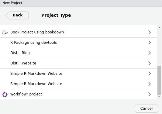
Choose
New Directoryand then scroll down the list of project types to selectworkflowr project. If you don’t see the workflowr project template, go to Troubleshooting.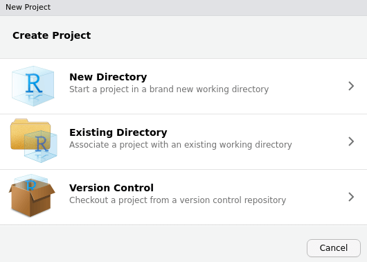
-
Type
myproject(or a more inventive name if you prefer) as the directory name, choose where to save it on your computer, and clickCreate Project.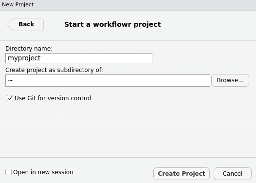
RStudio will create a workflowr project myproject and
opened the project in RStudio. Under the hood, RStudio is running a
workflowr command wflow_start() - so if you prefer to start
a new project from the console instead of using the RStudio menus then
you could use wflow_start().
Take a look at the workflowr directory structure in the Files pane, which should be something like this:
    myproject/
    |-- .gitignore
    |-- .Rprofile
    |-- _workflowr.yml
    |-- analysis/
    |   |-- about.Rmd
    |   |-- index.Rmd
    |   |-- license.Rmd
    |   |-- _site.yml
    |-- code/
    |   |-- README.md
    |-- data/
    |   |-- README.md
    |-- docs/
    |-- myproject.Rproj
    |-- output/
    |   |-- README.md
    |-- README.md
The most important directory for you to pay attention to now is the
analysis/ directory. This is where you should store all
your analyses as R Markdown (Rmd) files. Other directories created for
your convenience include data/ for storing data, and
code/ for storing long-running or supplemental code you
don’t want to include in an Rmd file. Note that the docs/
directory is where the website HTML files will be created and stored by
workflowr, and should not be edited by the user.
Build your website
The files and directories created by workflowr are already almost a
website! The only thing missing are the crucial html files.
Take a look in the docs/ directory where the html files for
your website need to be created… notice that it is sadly empty.
In workflowr the html files for your website are created in the
docs/ directory by knitting (or “building”) the
.Rmd files in the analysis/ directory. When
you knit or build those files – either by using the knitr button, or by
typing wflow_build() in the console – the resulting html
files are saved in the docs directory.
The docs/ directory is currently empty because we
haven’t run any of the .Rmd files yet. So now let’s run
these files. We will do it both ways, using both the knit button and
using wflow_build():
Open the file
analysis/index.Rmdand knit it now. You can open it by using the files pane, or by typingwflow_open("analysis/index.Rmd")in the R console. You knit the file by pressing the knit button in RStudio.There are also two other
.Rmdfiles in theanalysisdirectory. Build these by typingwflow_build()in the R console. This will build all the R Markdown files inanalysis/, and save the resulting html files indocs/. (Note, it won’t re-buildindex.Rmdbecause you have not changed it since running it before, so it does not need to.1
Ignore the warnings in the workflowr report for now; we will return to these later.
Collect some data!
To do an interesting analysis you will need some data. Here, instead
of doing a time-consuming experiment, we will use a convenient built-in
data set from R. While not the most realistic, this avoids any issues
with downloading data from the internet and saving it correctly. The
data set ToothGrowth contains the length of the teeth for
60 guinea pigs given 3 different doses of vitamin C either via orange
juice (OC) or directly with ascorbic acid
(VC).
-
To get a quick sense of the data set, run the following in the R console.
## len supp dose ## 1 4.2 VC 0.5 ## 2 11.5 VC 0.5 ## 3 7.3 VC 0.5 ## 4 5.8 VC 0.5 ## 5 6.4 VC 0.5 ## 6 10.0 VC 0.5summary(ToothGrowth)## len supp dose ## Min. : 4.20 OJ:30 Min. :0.500 ## 1st Qu.:13.07 VC:30 1st Qu.:0.500 ## Median :19.25 Median :1.000 ## Mean :18.81 Mean :1.167 ## 3rd Qu.:25.27 3rd Qu.:2.000 ## Max. :33.90 Max. :2.000str(ToothGrowth)## 'data.frame': 60 obs. of 3 variables: ## $ len : num 4.2 11.5 7.3 5.8 6.4 10 11.2 11.2 5.2 7 ... ## $ supp: Factor w/ 2 levels "OJ","VC": 2 2 2 2 2 2 2 2 2 2 ... ## $ dose: num 0.5 0.5 0.5 0.5 0.5 0.5 0.5 0.5 0.5 0.5 ... -
To mimic a real project that will have external data files, save the
ToothGrowthdata set to thedata/subdirectory usingwrite.csv().write.csv(ToothGrowth, file = "data/teeth.csv")
Understanding paths
Look at that last line of code. Where will the file be saved on your computer? To understand this very important issue you need to understand the idea of “relative paths” and “working directory”.
Before explaining these ideas, let us consider a different way we could have saved the file. Suppose we had typed
write.csv(ToothGrowth, file = "C:/Users/GraceHopper/Documents/myproject/data/teeth.csv")Then it is clear exactly where on the computer we want the file to be saved. Specifying the file location this very explicit way is called specifying the “full path” to the file. It is conceptually simple. But it is also a pain for many reasons – it is more typing, and (more importantly) if we move the project to a different computer it will likely no longer work because the paths will change!
Instead we typed
write.csv(ToothGrowth, file = "data/teeth.csv")Specifying the file location this way is called specifying the
“relative path” because it specifies the path to the file relative
to the current working directory. This means the full path to the
file will be obtained by appending the specified relative path to the
(full) path of the current working directory. For example, if the
current working directory is
C:/Users/GraceHopper/Documents/myproject/ then the file
will be saved to
C:/Users/GraceHopper/Documents/myproject/data/teeth.csv. If
the current working directory is C:/Users/Matt124/myproject
then the file will be saved to
C:/Users/Matt124/myproject/data/teeth.csv.
So, what is your current working directory? When you start or open a
workflowr project in RStudio (e.g. by clicking on
myproject.Rproj) RStudio will set the working directory to
the location of the workflowr project on your computer. So your current
working directory should be the location you chose when you started your
workflowr project. You can check this by typing getwd() in
the R console.
Notice how, by using relative paths, the code used here works for you whatever operating system you are on and however your computer is set up! You should always use relative paths where possible because it can help make your code easier for others to run and easier for you to run on different computers and different operating systems.
Create a new analysis
So, now we have some data, we are ready to perform a small analysis.
To start a new analysis in RStudio, use the wflow_open()
command.
-
In the R console, open a new R Markdown file by typing
wflow_open("analysis/teeth.Rmd")Notice that we again used a relative path! Relative paths are good for opening files as well as saving files. This command should create a new
.Rmdfile in theanalysissubdirectory of your workflowr project, and open it for editing in RStudio. The file looks pretty much like other.Rmdfiles, but in the header note that workflowr provides its own custom output format,workflowr::wflow_html. The other minor difference is thatwflow_open()adds the editor optionchunk_output_type: console, which causes the code to be executed in the R console instead of within the document. If you prefer the results of the code chunks be embedded inside the document while you perform the analysis, you can delete those lines (note that this has no effect on the final results, only on the display within RStudio). -
Copy the code chunk below and paste it at the bottom of the file
teeth.Rmd. The code imports the data set from the file you previously created2. Execute the code in the R console by clicking on the Run button or using the shortcutCtrl/CMD+Enter.```{r import-teeth} teeth <- read.csv("data/teeth.csv", row.names = 1) head(teeth) ```Note: if you copy and paste this chunk, make sure to remove any spaces before each of the backticks (
```) so that they will be correctly recognized as indicating the beginning and end of a code chunk. -
Next create some boxplots to explore the data. Copy the code chunk below and paste it at the bottom of the file
teeth.Rmd. Execute the code to see create the plots.```{r boxplots} boxplot(len ~ dose, data = teeth) boxplot(len ~ supp, data = teeth) boxplot(len ~ dose + supp, data = teeth) ``` -
To compare the tooth length of the guinea pigs given orange juice versus those given vitamin C, you could perform a permutation-based statistical test. This would involve comparing the observed difference in teeth length due to the supplement method to the observed differences calculated from random permutations of the data. The basic idea is that if the observed difference is an outlier compared to the differences generated after permuting the supplement method column, it is more likely to be a true signal not due to chance alone. We are not going to perform the full permutation test here, but we will just demonstrate the idea of a permutation. Copy the code chunk below, paste it at the bottom of of the file
teeth.Rmd, and execute it. Try executing it several times – does it give you a different answer each time?```{r permute} # Observed difference in teeth length due to supplement method mean(teeth$len[teeth$supp == "OJ"]) - mean(teeth$len[teeth$supp == "VC"]) # Permute the observations supp_perm <- sample(teeth$supp) # Calculate mean difference in permuted data mean(teeth$len[supp_perm == "OJ"]) - mean(teeth$len[supp_perm == "VC"]) ``` In the R console, run
wflow_build(). Note the value of the observed difference in the permuted data.-
In RStudio, click on the Knit button. Has the value of the observed difference in the permuted data changed? It should be identical. This is because workflowr always sets the same seed prior to running the analysis.3 To better understand this behavior as well as the other reproducibility safeguards and checks that workflowr performs for each analysis, click on the workflowr button at the top and select the “Checks” tab.
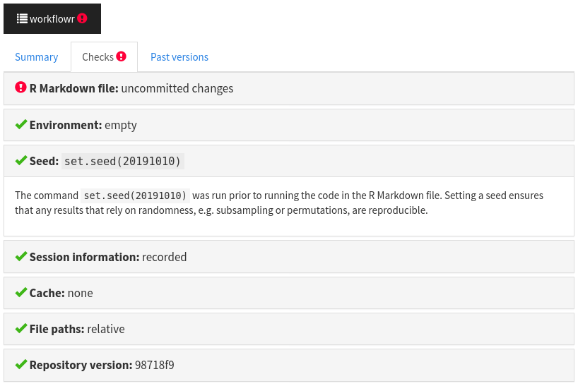
You can see the value of the seed that was set using
set.seed()before the code was executed.
Publish your analysis!
You should also notice that workflowr is still giving you a warning: it says you have “uncommitted changes” in your .Rmd file. The term “commit” is a term from version control: it basically means to save a snapshot of the current version of a file so that you could return to it later if you wanted (even if you changed or deleted the file in between).
So, workflowr is warning you that you haven’t saved a snapshot of your current analysis. If this analysis is something you are currently (somewhat) happy with then you should save a snapshot that will allow you to go back to it at any time in the future (even if you change the .Rmd file between now and then). In workflowr we use the term “publish” for this process: any analysis that you “publish” will be one that you can go back to in the future. You will see that it is pretty easy to publish an analysis so you should do it whenever you create a first working version, and whenever you make a change that you might want to keep. Don’t wait to think that it is your “final” version before publishing, or you will never publish!
-
Publish your analysis by typing:
wflow_publish("analysis/teeth.Rmd", message = "Analyze teeth growth")The function
wflow_publish()performs three steps: 1) commits (snapshots) the .Rmd files, 2) rebuilds the Rmd files to create the html file and figures, and 3) commits the HTML and figure files. This guarantees that the results in each html file is always generated from an exact, known version of the Rmd file (you can see this version embedded in the workflowr report). An informative message will help you find a particular version later. -
Open the workflowr report of
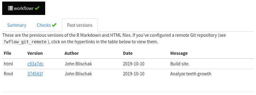
teeth.htmlby clicking on the button at the top of the page. Navigate to the tab “Past versions”. Note that the record of all past versions will be saved here. Once the project has been added to GitHub (you will do this in the next section), the “Past versions” tab will include hyperlinks for convenient viewing of the past versions of the Rmd and HTML files.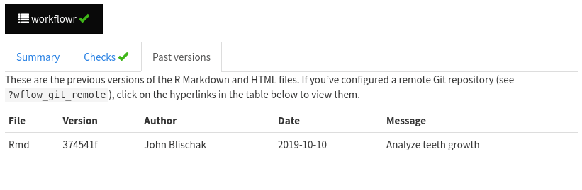
Checking your status
When you are working on several analyses over a period of time it can
be difficult to keep track of which ones need attention, etc. You can
use wflow_status() to check on all your files.
In the R console, run
wflow_status(). This will show you the status of each of the Rmd files in your workflowr project. You should see thatteeth.rmdhas status “Published” because you just published it. But the other.Rmdfiles have status “Unpublished” because you haven’t published them yet. Also you will notice a comment that the filedata/teeth.csvis “untracked”. This basically means that the data file has not had a snapshot kept, which is dangerous as our analyses obviously depend on the version of the data we use….-
In the R console, run the command below to “publish” these other files 4.
wflow_publish(c("analysis/*Rmd", "data/teeth.csv"), message = "Publish data and other files") Navigate to check html files in the
docsdirectory, you should find that they all have a green light and no warnings.And run
wflow_status()again to confirm all is OK. Everything is published!
Share your results
So, now you have a website, with an analysis in it. But it is only on your computer, not the internet. To share your website with the world we will use the free service GitHub Pages.
-
In the R console, run the function
wflow_use_github(). The only required argument is your GitHub username. The name of the repository will automatically be named the same as the directory containing the workflowr project, in this case “myproject”.wflow_use_github("your-github-username")When the function asks if you would like it to create the repository on GitHub for you, enter
1. This should open your web browser so that you can authenticate with GitHub and then give permission for workflowr to create the repository on your behalf. Additionally, this function connects to your local repository with the remote GitHub repository and inserts a link to the GitHub repository into the navigation bar. If this fails to create a GitHub repository, go to Troubleshooting. -
To update your workflowr website to use GitHub links to past versions of the files (as well as update the navigation bar to include the GitHub link), republish the files. (You would not have to do this in future)
wflow_publish(republish = TRUE) -
To send your project to GitHub, run
wflow_git_push(). This will prompt you for your GitHub username and password. If this fails, go to Troubleshooting. -
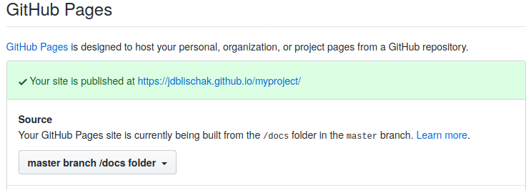
On GitHub, navigate to the Settings tab of your GitHub repository5. Scroll down to the section “GitHub Pages”. For Source choose “master branch /docs folder”. After it updates, scroll back down and click on the URL. If the URL doesn’t display your website, go to Troubleshooting.
Index your new analysis
Unfortunately your home page is not very inspiring. Also there is not
an easy want to find that nice analysis you did! A great way to keep
track of analyses and make them easy to find is to keep an index on your
website homepage. The homepage is created by
analysis/index.Rmd, so we are now going to edit this file
to add a link to our new analysis.
Open the file
analysis/index.Rmd. You can open it from the Files pane or runwflow_open("analysis/index.Rmd").-
Copy the line below and paste it at the bottom of the file
analysis/index.Rmd. This text uses “markdown” syntax to create a hyperlink to the tooth analysis. The text between the square brackets is displayed on the webpage, and the text in parentheses is the relative path to the teeth webpage. Note that you don’t need to include the subdirectorydocs/becauseindex.htmlandteeth.htmlare both already indocs/. (In an html file relative paths are specified relative to the current page which in this case will beindex.html.) Also note that you need to use the file extension.htmlsince that is the file that needs to be opened by the web browser.* [Teeth growth analysis](teeth.html) Maybe you would like to write a short introductory message in your index file e.g. “Welcome to my first workflowr website”!
You might also want to add a bit more details on what the tooth growth analysis did – a little detail in your index can be really helpful when it starts getting bigger…
Run
wflow_build()and then confirm that clicking on the link “Teeth growth” takes you to your teeth analysis page.Run
wflow_publish("analysis/index.Rmd")to publish this new index file.Run
wflow_status()to check everything is OK.Run
wflow_git_push()to push the changes to GitHub.-
Now go to your GitHub page again, and check out your website! (It can take a couple of minutes to refresh after pushing, so you may need to be patient). Navigate to the tooth analysis. Click on the links in the “Past versions” tab to see the past results. Click on the HTML hyperlink to view the past version of the HTML file. Click on the Rmd hyperlink to view the past version of the Rmd file on GitHub. Enjoy!
Conclusion
You have successfully created and shared a reproducible research
website. The key commands are a pretty short list:
wflow_build(), wflow_publish(),
wflow_status(), and wflow_git_push(). Using
the same workflowr commands, you can do the same for one of your own
research projects and share it with collaborators and colleagues.
To learn more about workflowr, you can read the following vignettes:
- Customize your research website
- Migrating an existing project to use workflowr
- How the workflowr package works
- Frequently asked questions
- Hosting workflowr websites using GitLab
- Sharing common code across analyses
- Alternative strategies for deploying workflowr websites
- Using large data files with workflowr
Troubleshooting
I don’t see the workflowr project as an available RStudio Project Type.
If you just installed workflowr, close and re-open RStudio. Also, make sure you scroll down to the bottom of the list.
The GitHub repository wasn’t created automatically by
wflow_use_github().
If wflow_use_github() failed unexpectedly when creating
the GitHub repository, or if you declined by entering n,
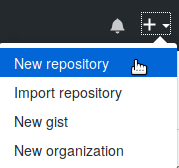
you can manually created the repository on GitHub. After logging in to
GitHub, click on the “+” in the top right of the page. Choose “New
repository”. For the repository name, type myproject. Do
not change any of the other settings. Click on the green button “Create
repository”. Once that is completed, you can return to the next step in
the tutorial.
I wasn’t able to push to GitHub with
wflow_git_push().
Unfortunately this function has a high failure rate because it relies
on the correct configuration of various system software dependencies. If
this fails, you can push to Git using another technique, but this will
require that you have previously installed Git on your computer. For
example, you can use the RStudio Git pane (click on the green arrow that
says “Push”). Alternatively, you can directly use Git by running
git push in the terminal.
The default behavior when
wflow_build()is run without any arguments is to build any R Markdown file that has been edited since its corresponding HTML file was last built.↩︎Note that the default working directory for a workflowr project is the root of the project. Hence the relative path is
data/teeth.csv. The working directory can be changed via the workflowr optionknit_root_dirin_workflowr.yml. See?wflow_htmlfor more details.↩︎Note that everyone in the workshop will have the same result because by default workflowr uses a seed that is the date the project was created as YYYYMMDD. You can change this by editing the file
_workflowr.yml.↩︎The command uses the wildcard character
*to match all the Rmd files inanalysis/. If this fails on your computer, try running the more verbose command:wflow_publish(c("analysis/index.Rmd", "data/teeth.csv"), message = "Analyze teeth growth")↩︎If your GitHub repository wasn’t automatically opened by
wflow_git_push(), you can manually enter the URL into the browser:https://github.com/username/myproject.↩︎